pacman::p_load(sf, tmap, tidyverse)In-class-7
mpsz <- st_read( dsn = "geospatial",
                layer = "MP14_SUBZONE_WEB_PL")
Reading layer `MP14_SUBZONE_WEB_PL' from data source
`D:\DaisyL12138\ISSS608-V\in-class\geospatial' using driver `ESRI Shapefile'
Simple feature collection with 323 features and 15 fields
Geometry type: MULTIPOLYGON
Dimension: XY
Bounding box: xmin: 2667.538 ymin: 15748.72 xmax: 56396.44 ymax: 50256.33
Projected CRS: SVY21popdata <- read_csv("respopagesextod2011to2020.csv")popdata2020 <- popdata %>%
filter(Time == 2020) %>%
group_by(PA, SZ,AG) %>%
summarise('POP' = sum(Pop),.groups = 'drop') %>%
ungroup()%>%
pivot_wider(names_from=AG,
values_from=POP) %>%
mutate(YOUNG = rowSums(.[3:6])
+rowSums(.[12])) %>%
mutate(ECONOMYACTIVE = rowSums(.[7:11])+rowSums(.[13:15]))%>%
mutate(AGED=rowSums(.[16:21])) %>%
mutate(TOTAL=rowSums(.[3:21])) %>%
mutate(DEPENDENCY = (YOUNG + AGED)/ECONOMYACTIVE) %>%
select(PA, SZ, YOUNG,
ECONOMYACTIVE, AGED,
TOTAL, DEPENDENCY)popdata2020 <- popdata2020 %>%
mutate_at(.vars = vars(PA, SZ), toupper) %>%
filter(ECONOMYACTIVE > 0)mpsz_pop2020 <- left_join(mpsz, popdata2020,
by = c("SUBZONE_N" = "SZ"))write_rds(mpsz_pop2020, "mpszpop2020.rds")tmap_mode("plot")
qtm(mpsz_pop2020,
fill = "DEPENDENCY")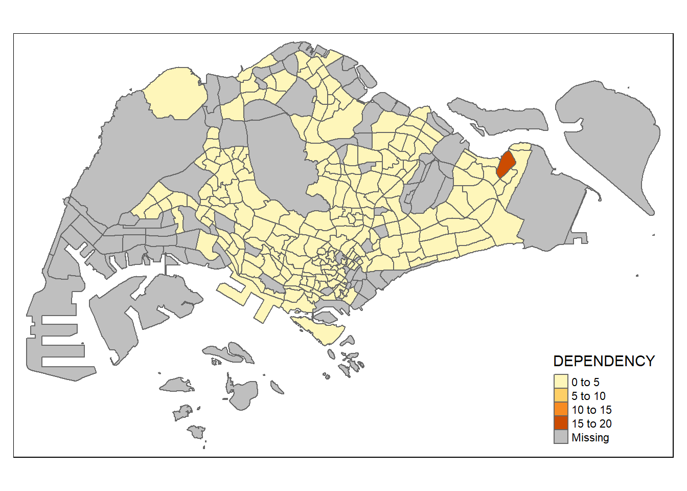
tm_shape(mpsz_pop2020)+
  tm_fill("DEPENDENCY",
          style = "quantile",
          palette = "Blues",
          title = "Dependency ratio") +
  tm_layout(main.title = "Distribution of Dependency Ratio by planning subzone",
            main.title.position = "center",
            main.title.size = 1.2,
            legend.height = 0.45,
            legend.width = 0.35,
            frame = TRUE) +
  tm_borders(alpha = 0.5) +
  tm_compass(type="8star", size = 2) +
  tm_scale_bar() +
  tm_grid(alpha =0.2) +
  tm_credits("Source: Planning Sub-zone boundary from Urban Redevelopment Authorithy (URA)\n and Population data from Department of Statistics DOS",
             position = c("left", "bottom"))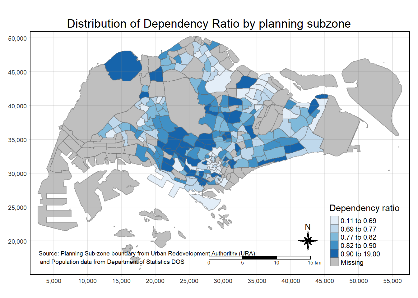
tm_shape(mpsz_pop2020) +
  tm_polygons()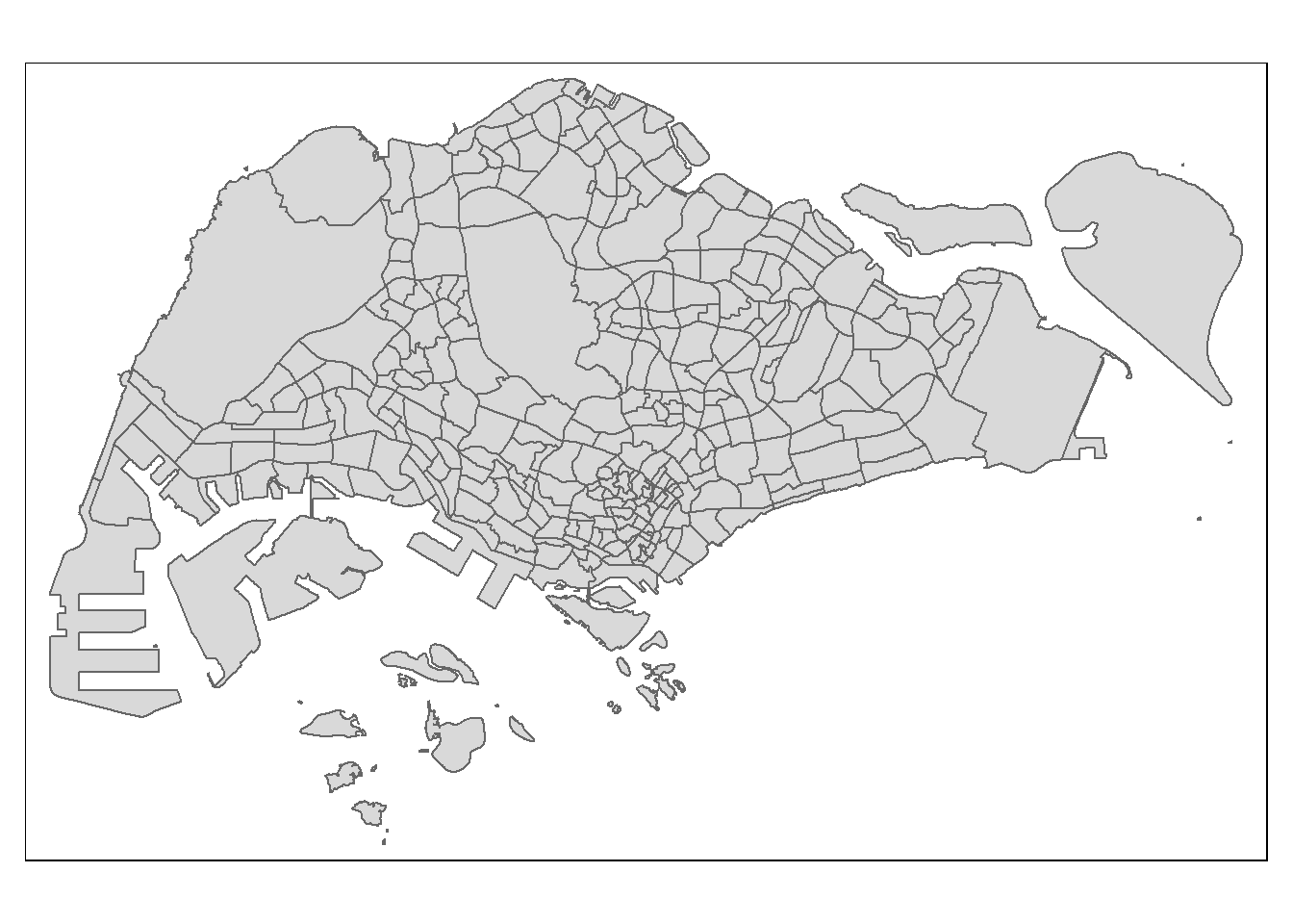
tm_shape(mpsz_pop2020)+
  tm_polygons("DEPENDENCY")
tm_shape(mpsz_pop2020)+
  tm_fill("DEPENDENCY")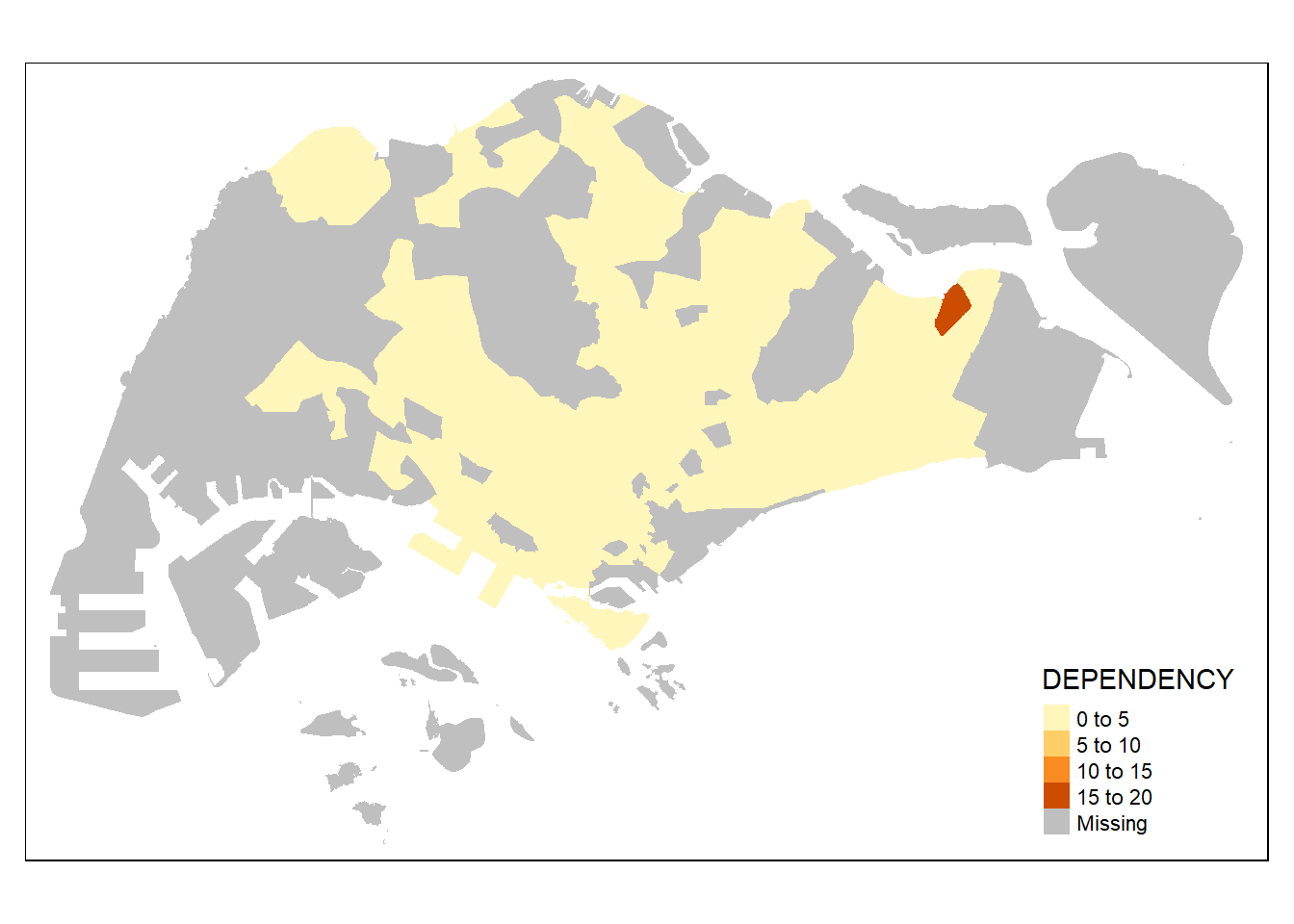
tm_shape(mpsz_pop2020)+
  tm_fill("DEPENDENCY",
          n = 5,
          style = "jenks") +
  tm_borders(alpha = 0.5)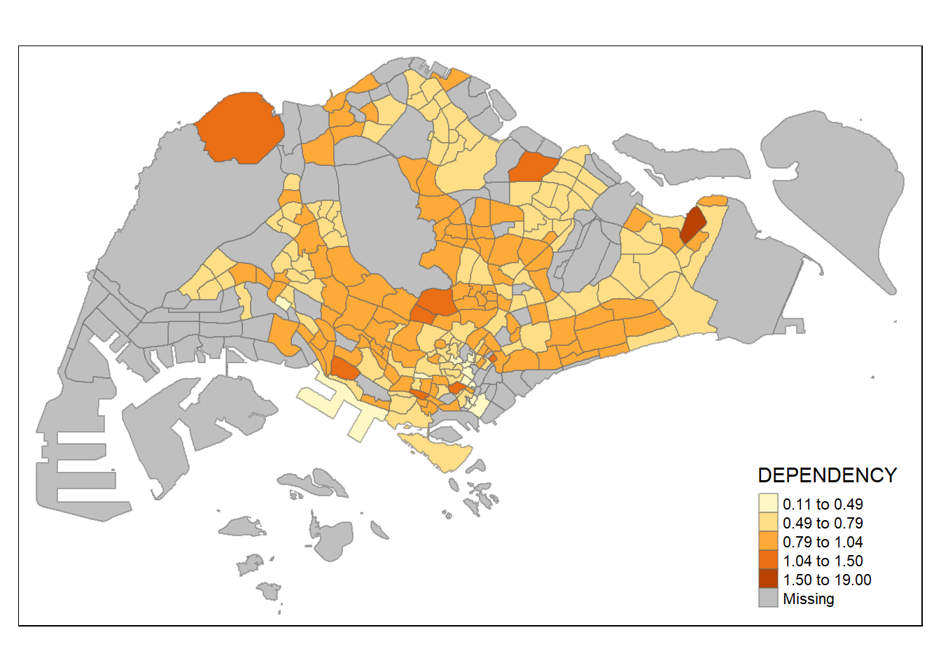
summary(mpsz_pop2020$DEPENDENCY) Min. 1st Qu. Median Mean 3rd Qu. Max. NA's
0.1111 0.7147 0.7866 0.8585 0.8763 19.0000 92 tm_shape(mpsz_pop2020)+
tm_fill("DEPENDENCY",
breaks = c(0, 0.60, 0.70, 0.80, 0.90, 1.00)) +
tm_borders(alpha = 0.5)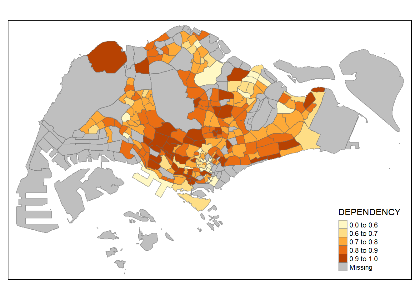
tm_shape(mpsz_pop2020)+
  tm_fill("DEPENDENCY",
          style = "quantile",
          palette = "Greens") +
  tm_borders(alpha = 0.5)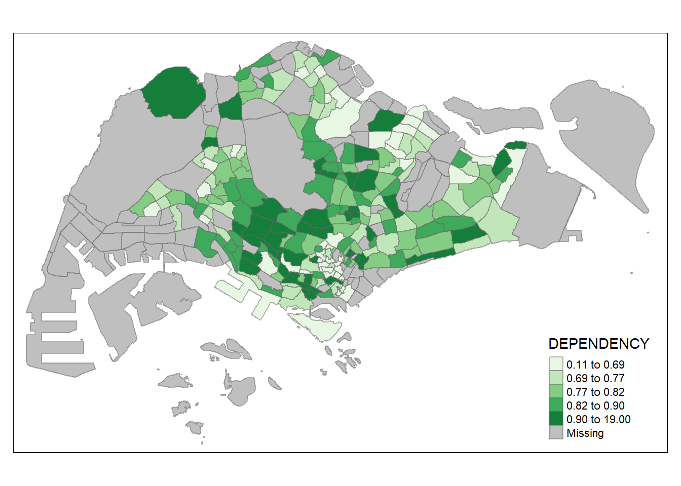
tm_shape(mpsz_pop2020)+
  tm_fill("DEPENDENCY",
          style = "quantile",
          palette = "-Greens") +
  tm_borders(alpha = 0.5)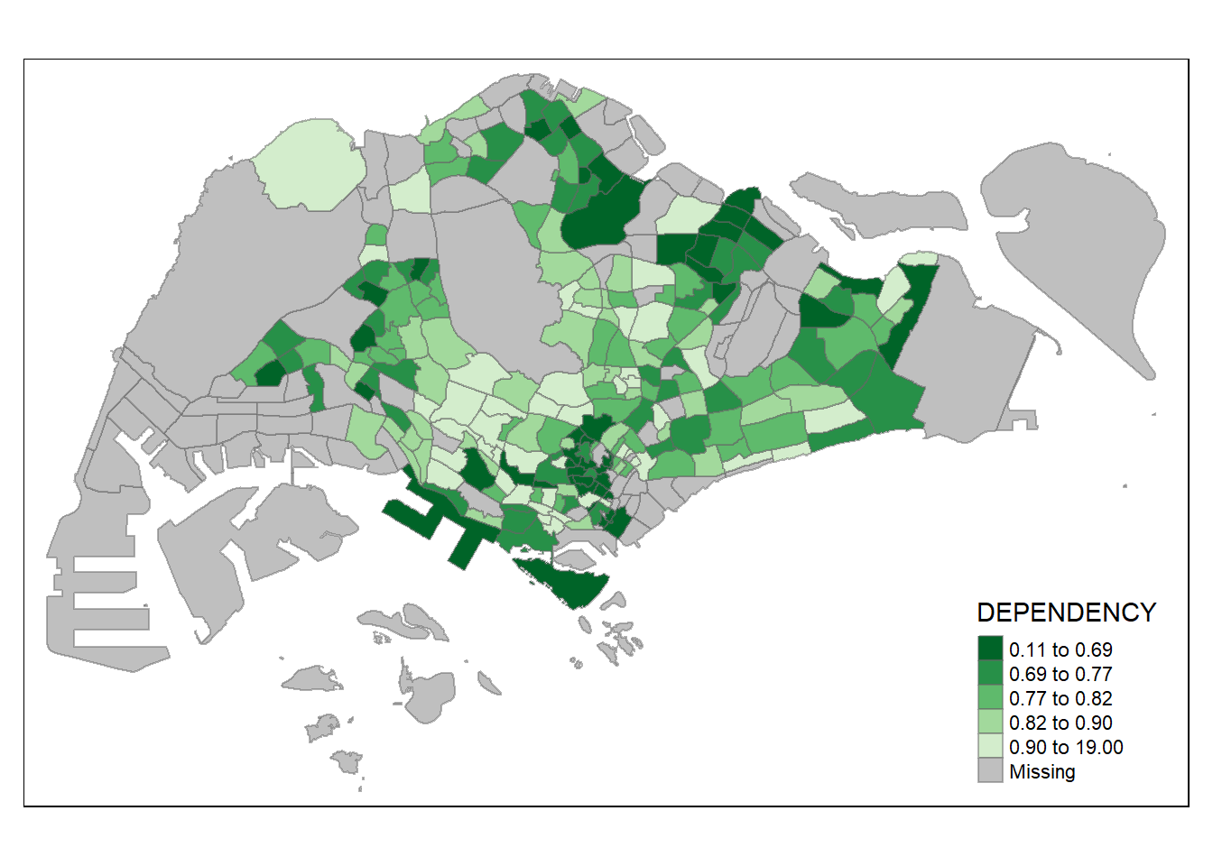
tm_shape(mpsz_pop2020)+
  tm_fill("DEPENDENCY",
          style = "jenks",
          palette = "Blues",
          legend.hist = TRUE,
          legend.is.portrait = TRUE,
          legend.hist.z = 0.1) +
  tm_layout(main.title = "Distribution of Dependency Ratio by planning subzone \n(Jenks classification)",
            main.title.position = "center",
            main.title.size = 1,
            legend.height = 0.45,
            legend.width = 0.35,
            legend.outside = FALSE,
            legend.position = c("right", "bottom"),
            frame = FALSE) +
  tm_borders(alpha = 0.5)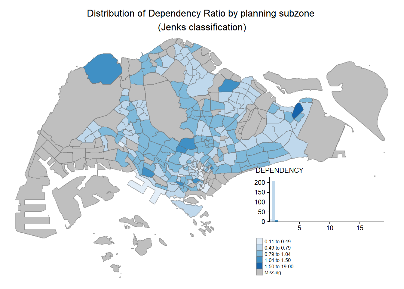
tm_shape(mpsz_pop2020)+
  tm_fill(c("YOUNG", "AGED"),
          style = "equal",
          palette = "Blues",
          ncols=2) +
  tm_layout(legend.position = c("right", "bottom")) +
  tm_borders(alpha = 0.5) +
  tmap_style("white")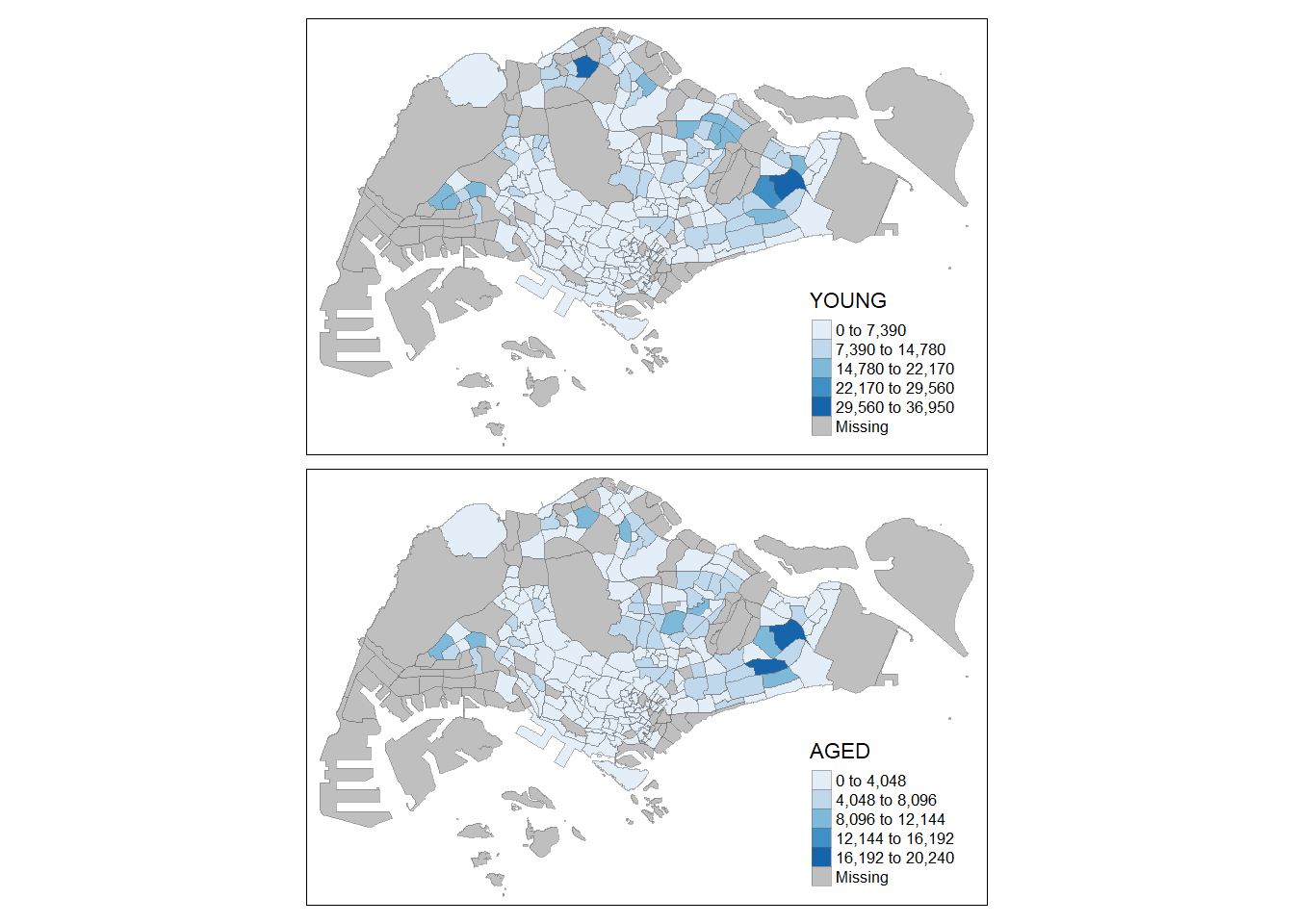
tm_shape(mpsz_pop2020) +
  tm_fill("DEPENDENCY",
          style = "quantile",
          palette = "Blues",
          thres.poly = 0) +
  tm_facets(by="REGION_N",
            free.coords=TRUE,
            drop.shapes=TRUE) +
  tm_layout(legend.show = FALSE,
            title.position = c("center", "center"),
            title.size = 20) +
  tm_borders(alpha = 0.5)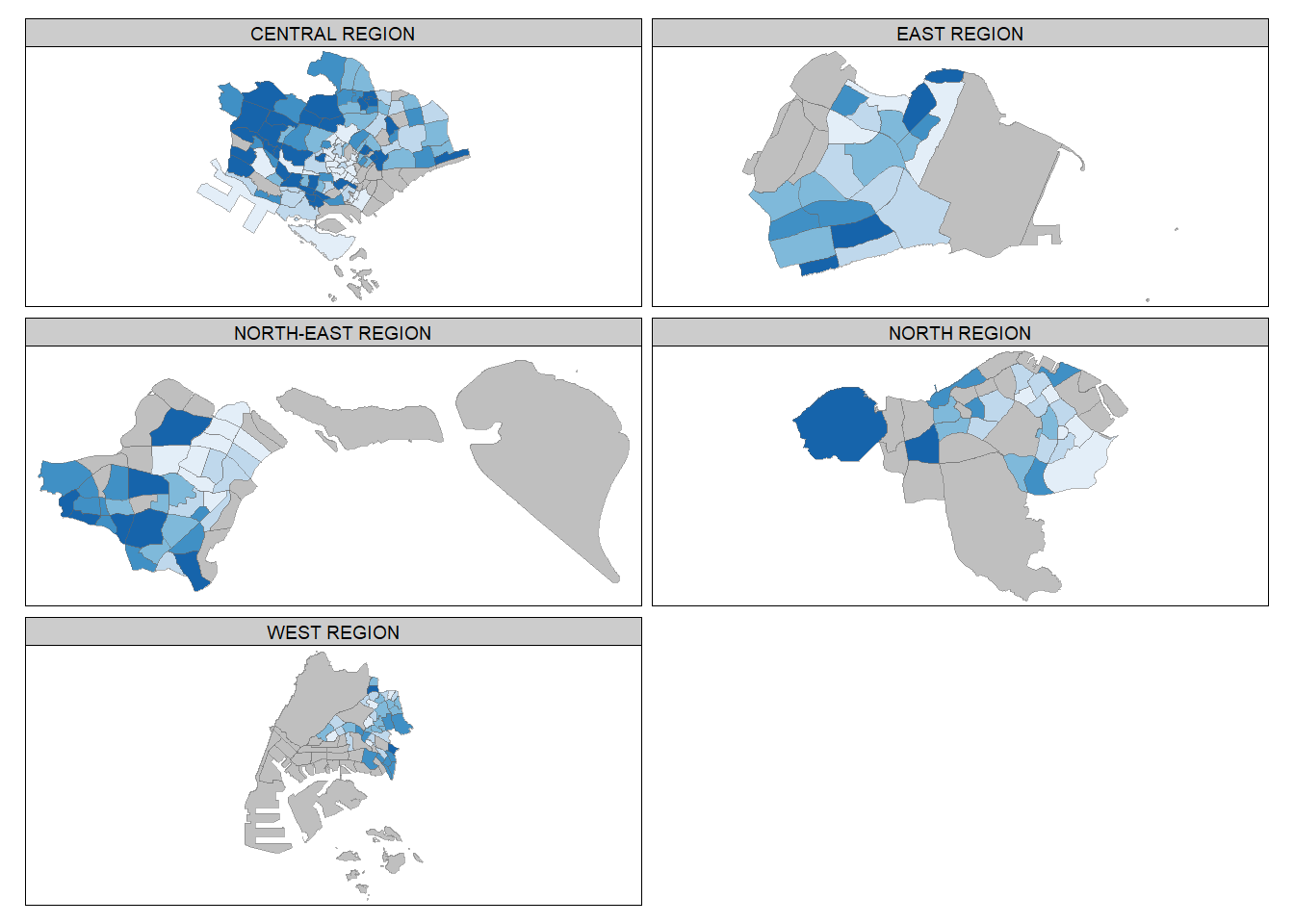
tm_shape(mpsz_pop2020[mpsz_pop2020$REGION_N=="CENTRAL REGION", ])+
  tm_fill("DEPENDENCY",
          style = "quantile",
          palette = "Blues",
          legend.hist = TRUE,
          legend.is.portrait = TRUE,
          legend.hist.z = 0.1) +
  tm_layout(legend.outside = TRUE,
            legend.height = 0.45,
            legend.width = 5.0,
            legend.position = c("right", "bottom"),
            frame = FALSE) +
  tm_borders(alpha = 0.5)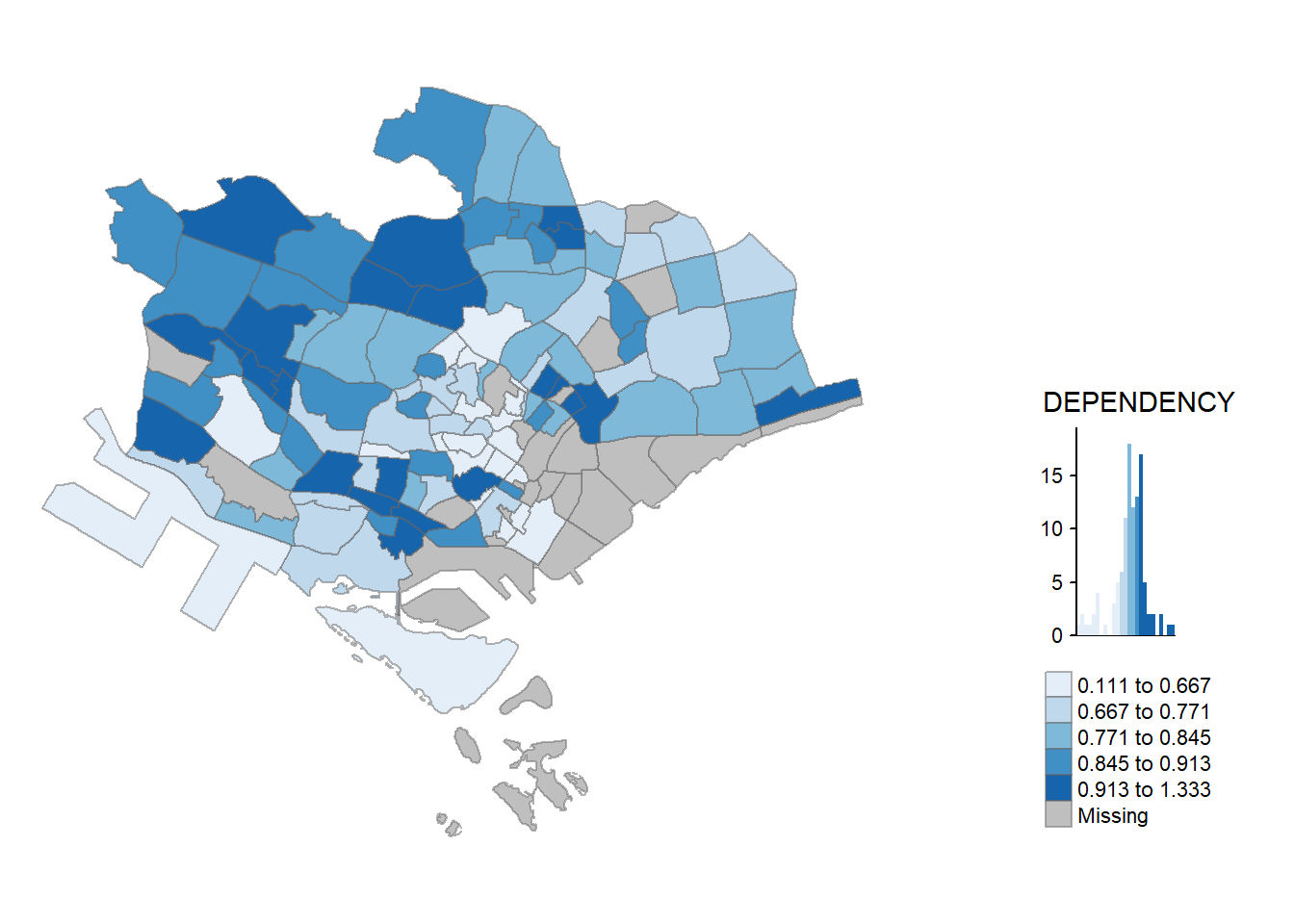
library(tmap)
data("World")

tm_shape(World) +
    tm_polygons("HPI")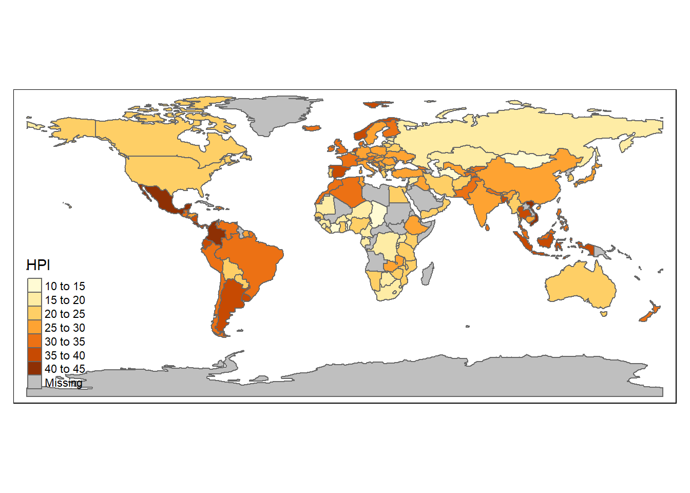
tmap_mode("view")

tm_shape(World) +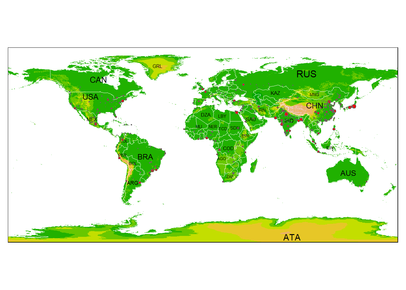
tm_polygons("HPI")data(World, metro, rivers, land)
tmap_mode("plot")
## tmap mode set to plotting
tm_shape(land) +
tm_raster("elevation", palette = terrain.colors(10)) +
tm_shape(World) +
tm_borders("white", lwd = .5) +
tm_text("iso_a3", size = "AREA") +
tm_shape(metro) +
tm_symbols(col = "red", size = "pop2020", scale = .5) +
tm_legend(show = FALSE)